Page 5 - Demo
P. 5


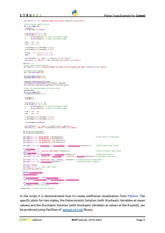
                                    Planar Truss Example for Comrel Add-on RCP Consult, 2019-2026 Page 5 plt.text(12.0, 8.0, 'Internal member forces [N]',fontsize=16,ha='center') # Plot internal member force N for e in range(nfe): l=leng[e]/2 n=np.abs(N[e])*0.0000005 X=np.array([-l, l, l, -l]) Y=np.array([-n, -n, n, n]) c = np.cos(theta[e]) # cosine inclination angle s = np.sin(theta[e]) # sinus inclination angle Xrot = X*c - Y*s Yrot = X*s + Y*c x=(XY[IEN[e,0],0]+XY[IEN[e,1],0])/2 y=(XY[IEN[e,0],1]+XY[IEN[e,1],1])/2 if(N[e] >= 0): co=(1.0, 0.6, 0.5) else : co=(0.5, 0.6, 1.0) plt.fill(Xrot + x, Yrot + y, color=co, ec='0', lw=0.5) plt.text(x, y, '%0.1f N' % N[e],fontsize=7,ha='center',va='center') elif nf == 2: # Set a main subtitle of plot plt.text(12.0, 8.0, r'Internal member von Mises stress $\\sigma_{v}$ [MPa]',fontsize=16,ha='center') # Prepare color mapping jet = plt.get_cmap('jet') minA=min(abs(N/area*1e-6)) maxA=max(abs(N/area*1e-6)) cNorm=plt.Normalize(minA, maxA) scalarMap=cmx.ScalarMappable(norm=cNorm, cmap=jet) plt.colorbar(scalarMap,use_gridspec=True,ax=plt.gca()) # Plot for internal member von Mises stress dA=maxA-minA for e in range(nfe): Su=abs(N[e]/area[e]*1e-6) l=leng[e]/2 n=Su/dA*0.2 X=np.array([-l, l, l, -l]) Y=np.array([-n, -n, n, n]) c = np.cos(theta[e]) # cosine inclination angle s = np.sin(theta[e]) # sinus inclination angle Xrot = X*c - Y*s Yrot = X*s + Y*c x=(XY[IEN[e,0],0]+XY[IEN[e,1],0])/2 y=(XY[IEN[e,0],1]+XY[IEN[e,1],1])/2 co=scalarMap.to_rgba(Su) plt.fill(Xrot + x, Yrot + y, color=co,lw=0.5,alpha=0.7) plt.text(x, y, '%0.0f' % Su,fontsize=7,ha='center',va='center') ## Do rest for all plots plt.title(tit,fontsize=18) plt.text(22, 5.5, 'A1=%g $m^2
   1   2   3   4   5   6   7   8   9   10


% A1,fontsize=8) # plot values of input data plt.text(22, 5.2, 'A2=%g $m^2
   1   2   3   4   5   6   7   8   9   10


% A2,fontsize=8) plt.text(22, 4.9, 'E1=%g $N/m^2
   1   2   3   4   5   6   7   8   9   10


% E1,fontsize=8) plt.text(22, 4.6, 'E2=%g $N/m^2
   1   2   3   4   5   6   7   8   9   10


% E2,fontsize=8) plt.text(-1.0, 5.5, StrurelName+' '+StrurelModule+' '+StrurelVersion,fontsize=12) # plot a main title of plot if StrurelMode == 0: plt.text(-1.0, 5.0, 'State at Mean Values',fontsize=10) # data at state of mean values elif StrurelMode == 2: plt.text(-1.0, 5.0, StrurelIMET+', '+StrurelIOPT,fontsize=10) # data at beta-point plt.text(-1.0, 4.5, 'beta=%.5f' % StrurelBeta+', '+'Pf=%.5f' % StrurelPf,fontsize=10) # calculated beta and Pf plt.text(-1.9, 9.7, 'matplotlib '+mpl.__version__, fontsize=7) # invoked version of matplotlib plt.text(-1.9, -1.8, StrurelEngine,fontsize=7) # invoked version of engine plt.axis('scaled') plt.axis([-2, 26, -2, 10]) # plot frame plt.grid(True,alpha=0.3) global StrurelPlotCount StrurelPlotCount+=1 if StrurelPlotMode == 2 or StrurelPlotMode == 3: plt.savefig(StrurelPlotName+str(StrurelPlotCount)+StrurelPlotType) if StrurelPlotMode == 1 or StrurelPlotMode == 3: plt.show() # end of plot blockreturn uout # return value of functionIn the script it is demonstrated how to create additional visualization from Python. The specific plots for two states, the Deterministic Solution (with Stochastic Variables at mean values) and the Stochastic Solution (with Stochastic Variables at values at the %u00df-point), can be produced using facilities of matplotlib library.
   1   2   3   4   5   6   7   8   9   10